## Abstract PM_2.5 pollution imposes substantial health risks on urban residents. Previous studies mainly focused on assessing peoples’ exposures at static locations, such as homes or workplaces. There has been a scarcity of research that quantifies the dynamic PM_2.5 exposures of people when they travel in cities. To address this gap, we use cellphone positioning data and PM_2.5 concentration data collected from smart sensors along roads in Guangzhou, China, to assess personal travel exposure to on-road PM_2.5. First, we extract the trips of cellphone users from their trajectories and use the shortest path algorithm to calculate their travel routes on the road network. Second, the travel exposure of each user is estimated by associating their movement patterns with PM_2.5 concentrations on roads. The result shows that most users’ average travel exposures per hour fall within the range of 20 μg/m³ to 75 μg/m³. Travel exposure varies across users, and 54.0% of users experience low travel exposure throughout the day, 25.5% of users experience high travel exposure in the evening, and 20.5% of users experience high travel exposure in the afternoon. Furthermore, the impacts of on-road PM_2.5 on urban populations are uneven across roads. More attention should be given to roads with high PM_2.5 concentrations and traffic flows in each period, such as Huan Shi Middle Road in the morning, Inner Ring Road in the afternoon, and Xinjiao Middle Road in the evening. The findings in this study can contribute to a more in-depth understanding of the relationship between air pollution and the travel activities of urban populations. **Keywords:** Travel exposure; On-road PM2.5 concentrations; Cellphone positioning data; Mobile sensors ## 1. Introduction With economic development and increased car ownership in many Chinese cities, vehicle emissions (e.g., particulate matter, nitrogen oxides, carbon monoxide, and volatile organic compounds) have become a prominent source of urban air pollution in recent years (China Vehicle Environmental Management Annual Report, 2018). Among different traffic-related air pollutants, PM_2.5 is the most detrimental to human health (Bowatte et al., 2015) because it can cause respiratory and cardiovascular issues even at very low concentrations (Chen et al., 2008; Cohen et al., 2017; Dominici et al., 2006). Personal PM_2.5 exposure assessment studies have received considerable attention from the perspectives of health geography and public health. However, most previous studies mainly focused on examining peoples’ exposure at their homes or workplaces and have neglected the risks from dynamic exposure along roads when they travel in the city. Although most people spend relatively small amounts of their time travelling, travel exposure to PM_2.5 still comprises a disproportionately large portion of the individual exposures to air pollution (Gulliver and Briggs, 2005; Kwan et al., 2015; Park, 2020; Xu et al., 2019). Therefore, it is necessary to assess urban populations’ travel exposure to PM_2.5 on their daily travel routes. Previous literature on personal PM_2.5 exposure can be broadly categorized into static residence-based, mobility-based, and big databased approaches. The static residence-based approach assumes that people stay at home for the duration of the study. The exposures of people are assessed by utilizing the PM_2.5 concentrations at their residential locations. Thus, a considerable part of the literature has focused on accurately measuring PM_2.5 concentrations at different locations. The commonly used methods include proximity to sources or monitors (Wu et al., 2011), dispersion models (Andersson et al., 2021; Park, 2020), remote sensing-based approaches (He et al., 2021; Song et al., 2019), and spatial interpolation methods (Liu et al., 2017; Ouyang et al., 2018). However, the static residence-based approach ignores the mobility dynamics of individuals. An individual engages in an average of three to four out-of-home activities each day (Yin et al., 2018), and the air quality levels vary substantially across different activity locations (Kwan et al., 2015). Therefore, the air pollution exposures that are calculated by this approach significantly deviate from the actual exposures in people’s daily lives. More recent studies have focused on mobility-based exposure assessments, which aim to consider human mobility. Global positioning system (GPS) devices or travel surveys have been utilized to obtain human mobility data (Ma et al., 2020; Song et al., 2021; Yoo et al., 2015). In some research, the PM_2.5 concentration data were collected by sparsely and unevenly distributed monitoring stations. For instance, Yoo et al. (2015) used GPS-equipped cellphones to track the locations and activities of 43 participants throughout the day and estimated the daily exposures of participants by using a dynamic time-activity-based approach. They found that the exposure results differed substantially from those obtained with a static residence-based approach when individuals spent much time away from home. Song et al. (2021) evaluated the dynamic characteristics of the inhaled PM_2.5 doses of 984 residents over 24 h during workdays. In their research, the temporal and spatial characteristics of the inhaled PM_2.5 doses were closely related to the rhythms of people’s daily activities. Since sparse and unevenly distributed monitoring stations can lead to inaccurate estimates of ambient PM_2.5 concentrations, portable air pollution sensors have been increasingly used in geographic and epidemiological research (Birenboim et al., 2021; Ma et al., 2020; Piedrahita et al., 2014; Zhou and Lin, 2019). For instance, Ma et al. (2020) recruited 117 residents and collected their GPS trajectories and real-time PM_2.5 concentrations by using GPS tracking devices and smart air pollutant sensors. Portable air pollution sensors can obtain more accurate PM_2.5 concentration data than static monitoring stations. Therefore, the variations in individual PM_2.5 exposures at different activity locations (e.g., homes, workplaces, shops, and outdoor locations) and for different travel modes (e.g., walking, cycling, public transport, and private cars) can be investigated. Nevertheless, the number of samples in these studies is usually small, and acquiring travel surveys for large urban populations is costly and challenging. Location-based big data provide a practical means to assess the personal air pollution exposures of large populations (Dewulf et al., 2016; Guo et al., 2020; Li et al., 2019; Nyhan et al., 2016, 2019; Yu et al., 2018). On the one hand, the dynamic nature of location-based data can improve the biases in residence-based exposure estimations (Dewulf et al., 2016; Li et al., 2019; Yu et al., 2018). Dewulf et al. (2016) introduced cellphone data to air pollution exposure studies for the first time. The cellphone data and air pollution concentration data were combined to dynamically estimate the air pollution exposures. The mean exposures increased by 4.3% during the week and by 0.4% during the weekend when incorporating individual travel patterns. On the other hand, when compared with travel surveys, location-based big data have larger user scales and more widespread spatial coverage. For example, the dataset used in Nyhan et al. (2019) consisted of 607 million records that corresponded to approximately 1.2 million individual mobile phones in Eastern Massachusetts. Individual air pollution exposures could therefore be quantified by using mobile devices for populations of unprecedented size. The abovementioned research provides a glimpse into the rich literature that has examined personal air pollution exposures. Most of these studies have focused on assessing the exposures of individuals at static locations, such as homes or workplaces. However, very little knowledge is available on the dynamic exposures of people during travel. What are the major travel exposure patterns of urban populations? Although Xu et al. (2019) considered travel exposures in their study, the PM_2.5 concentrations were obtained by sparse monitoring stations and could not accurately capture the space-time dynamics of air pollution on roads. To answer this question, we combine cellphone positioning data and PM_2.5 concentration data collected from smart mobile sensors along roads to assess personal travel exposure to on-road PM_2.5. First, we extract the trips of cellphone users from their trajectories and use the shortest path algorithm to calculate their travel routes on the road network. Second, the travel exposures for each user are estimated by associating their movement patterns with PM_2.5 concentrations on roads. This research can enhance our understanding of the relationship between air pollution and the travel activities of urban populations. It can also provide targeted policies and valuable suggestions for the government and individuals to reduce the health risks caused by on-road PM_2.5 pollution. The remainder of this paper is organized as follows. Section 2 introduces the study area and data used. Section 3 describes the methodology, including estimating the spatial concentrations of on-road PM_2.5, trip identification and route simulations based on cellphone positioning data, and travel exposure estimations of cellphone users. The experimental results and analysis are presented in section 4. Section 5 discusses the validity of the shortest path assumption we made for simulating cellphone users’ travel routes. The final section provides concluding remarks and future research directions. ## 2. Study area and data ### 2.1. Study area Guangzhou is located in the northern part of the Pearl River Delta, and it is one of the most developed and densely populated cities in China. The total car ownership in Guangzhou reached 2.39 million in 2017 (Guangzhou Statistical Yearbook, 2018). The traffic-related pollution that is caused by road vehicle emissions is therefore nonnegligible. Moreover, Guangzhou has a dry season from October to March due to its maritime subtropical monsoon climate. Atmospheric inversions that hinder the diffusion of atmospheric pollutants are frequent during this time. 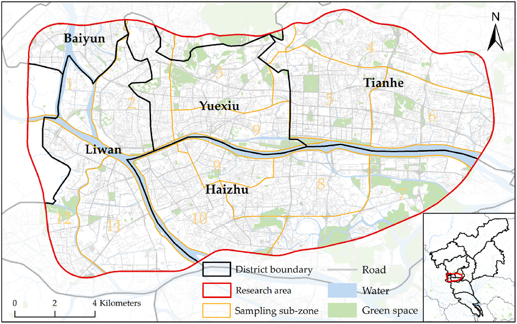Therefore, the air quality is poor compared with other seasons. This study focuses on five central city areas within the Guangzhou Outer Ring Road, including Yuexiu District, Haizhu District, Liwan District, Tianhe District, and Baiyun District. They are core areas of Guangzhou with highly developed transportation networks and densely populated residences (Fig. 1).

Figure 1. Research area. — **Figure 1.** Research area.

### 2.2. Dataset This study uses on-road PM_2.5 concentration data, cellphone positioning data, road network data, and housing price data collected in Guangzhou, China. The on-road PM_2.5 concentration data were collected by 36 cycling volunteers on November 27, 2017, using mobile air pollution monitoring sensors (AirBeam from HabitatMap). Before collecting data, all mobile monitoring sensors were tested and calibrated with a national fixed monitoring station. The test place is on the top floor (7F) of the Guangzhou municipal monitoring building on a sunny day. We conducted 8 h of continuous data observation from 9:00 to 17:00. All mobile monitoring sensors were placed in the same environment as the fixed monitoring station to eliminate the bias caused by different observation environments. Next, we calibrated the PM_2.5 concentration data collected by our mobile monitoring sensors with the data measured by the fixed monitoring station. First, we excluded the data of the first 5 min from the time the mobile sensors were turned on because these data can be unstable. Second, we averaged the data collected by each type of equipment at 5-min intervals and built a regression model for each mobile sensor to explore the relationship between the data collected by this mobile monitoring sensor and the data from the fixed monitoring station. The R² values of all regression models ranged from 0.58 to 0.90, with an average R² of 0.69. The detailed settings for PM_2.5 concentration data collection are shown in Zhou and Lin (2019). The research area was divided into twelve sampling subzones, in which the volunteers cycled to obtain the on-road PM_2.5 concentrations on the main roads in three periods: morning (7:00–12:00), afternoon (12:00–17:00) and evening (17:00–22:00). Each subzone was covered by three volunteers who took turns riding bicycles 2 to 3 times at speeds of 4–5 km/h. Finally, 428,000 valid PM_2.5 concentration records were obtained. We then corrected the data collected by each mobile monitoring sensor according to its corresponding regression model. 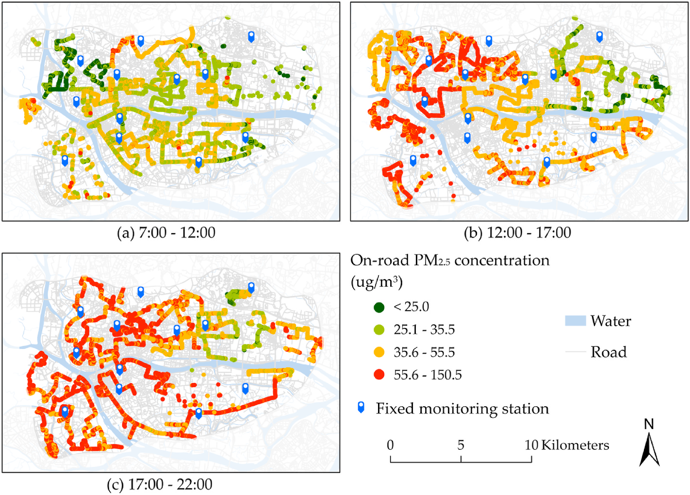The spatial distributions of the on-road PM_2.5 concentrations collected by the calibrated mobile monitoring sensors and the locations of ten national fixed monitoring stations are shown in Fig. 2. 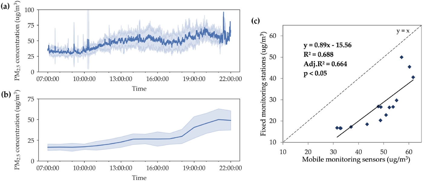The PM_2.5 concentrations of our mobile monitoring sensors and ten national fixed monitoring stations over time are illustrated in Fig. 3(a) and Fig. 3(b), respectively. The two curves have a similar trend, both increasing from morning until evening. Then, the Pearson correlation coefficients between them were calculated. As shown in Fig. 3(c), the adjusted R² was 0.66 (p < 0.05), which indicates that the on-road PM_2.5 concentration data that were collected by mobile monitoring sensors have good reliability. It should be noted that the PM_2.5 concentrations collected by the mobile monitoring sensors are higher than those collected by the fixed monitoring stations. This might be caused by the different observation characteristics between these two types of measurements. First, our mobile monitoring sensors were carried by the cycling volunteers, and they are mainly used to measure air pollution in a small area along the roads. In contrast, national fixed monitoring stations are usually set up in an open area, and the coverage area of each station is generally a radius of tens of kilometers (Ministry of Environmental Protection, 2013), and they are mainly used for regional air quality measurement. Second, the observation heights of the mobile monitoring sensors are less than 2 m above ground level, whereas the national fixed stations are usually located at heights of 3–15 m above the ground (Ministry of Environmental Protection, 2013). As mentioned in section 2.1, in the winter in Guangzhou, air pollutants can be easily suppressed near the ground because of atmospheric inversions, resulting in inconsistent PM_2.5 concentrations in the air at different heights. The observation heights of the mobile monitoring sensors are the heights of the daily exposure environments of urban residents. Thus, the PM_2.5 concentrations that were collected by the mobile monitoring sensors are more consistent with the actual exposure environments of residents’ travel activities.

Figure 2. The spatial distributions of on-road PM2.5 concentrations collected from mobile monitoring sensors during three periods. — **Figure 2.** The spatial distributions of on-road PM_2.5 concentrations collected from mobile monitoring sensors during three periods.

Figure 3. (a) PM2.5 concentrations of ten national fixed monitoring stations; (b) PM2.5 concentrations of mobile monitoring sensors; (c) Comparison of mobile monitoring sensors and fixed monitoring stations. — **Figure 3.** (a) PM_2.5 concentrations of ten national fixed monitoring stations; (b) PM_2.5 concentrations of mobile monitoring sensors; (c) Comparison of mobile monitoring sensors and fixed monitoring stations.

The cellphone positioning data were acquired from a major cellular operator in Guangzhou. The positions of the cellphone users were recorded at hourly intervals. The dataset contained data from 5.09 million phone users (approximately 36% of the total population) for one workday in December 2016. The number of records in the dataset is nearly 52.1 million, and each record contains information on the anonymous user ID, recording time, and longitude and latitude of the ambient cellphone towers communicating with the cellphones. Users whose trajectories were outside the study area were excluded. Furthermore, duplicate and abnormal records (e.g., adjacent records with speeds over 80 km/h and continuous missing data durations longer than 4 h) were deleted to ensure data quality. The locations derived from the cellphone positioning data could be recorded back and forth between cellphone towers (a.k.a. ping-pong effect) and could even be lost when the signal strength of the cellphone towers around the users was weak. Then, the ping-pong effects in the cellphone positioning data were eliminated using the point-clustering method proposed by Xu et al. (2020). Finally, the nearest neighbor interpolation method (Hoteit et al., 2014; Li et al., 2019, 2021) was utilized to fill in the missing locations of the cellphone user trajectories at hourly intervals. Then, a missing record could be interpolated by the value of its nearest sampling position in time. The urban road network data were obtained from Baidu Map, which is the largest map service provider in China. The data include 34,586 urban expressways, arterial roads, collector roads, and other road types. ## 3. Methods ### 3.1. Estimating the spatial concentration of on-road PM_2.5 To measure the PM_2.5 concentrations on roads at a fine scale, we divided each road into 10-m segments and calculated the mean PM_2.5 concentration for each segment. Since the mobile monitoring data did not cover all road segments in the study area, the kriging interpolation method (Wong et al., 2004) was utilized to estimate the PM_2.5 concentrations on those road segments without sampling points. Kriging interpolation was conducted for each period (i.e., morning, afternoon, and evening). The parameters of kriging interpolation were optimized by using leave-one-out cross validation. 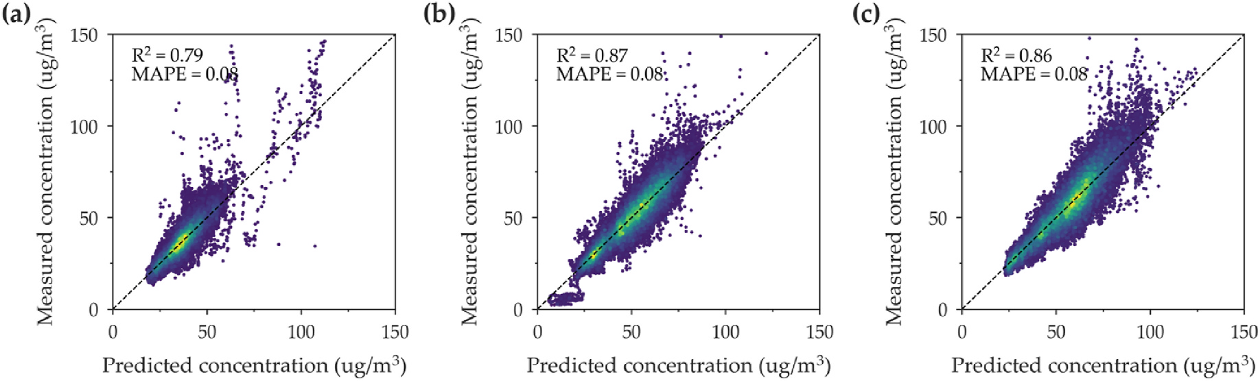The interpolation results were evaluated using the metrics of R² and the mean absolute percentage error (MAPE). Fig. 4 shows the measured and predicted on-road PM_2.5 concentrations in three periods. The R² values for the morning, afternoon, and evening periods are 0.79, 0.87, and 0.86, respectively. The MAPE values were stable at 0.08 in three periods. Overall, the interpolation results show good performance. After interpolation, we obtained the spatial distributions of the PM_2.5 concentrations for each period with a spatial resolution of 2 m × 2 m. Then, the PM_2.5 concentrations on road segments without sampling points were represented by the average PM_2.5 concentrations within a 50 m radius. 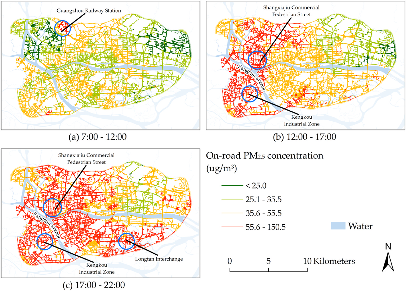The interpolated PM_2.5 concentrations on the road network of the study area are shown in Fig. 5. According to the air quality standards of the U.S. Environmental Protection Agency (U.S. EPA, 2012), PM_2.5 concentrations greater than 55.5 μg/m³ are considered “unhealthy” levels. As shown in Fig. 5, there are many roads with PM_2.5 concentrations above the “unhealthy” level in the afternoon and evening, which indicates that the potential exposure risks of residents cannot be ignored. The on-road PM_2.5 concentrations in the study area are high in the west and south and low in the east and north. The high-risk areas for PM_2.5 pollution are mainly located in commercial centers, transportation facilities, and industrial zones, such as Shangxiajiu Commercial Pedestrian Street, Guangzhou Railway Station, Fangcun Avenue, Longtan Interchange, and Kengkou Industrial Zone (Fig. 5).

Figure 4. Measured and predicted on-road PM2.5 concentrations in three periods. — **Figure 4.** Measured and predicted on-road PM_2.5 concentrations in three periods.

Figure 5. On-road PM2.5 concentrations in the study area during the three time periods. — **Figure 5.** On-road PM_2.5 concentrations in the study area during the three time periods.

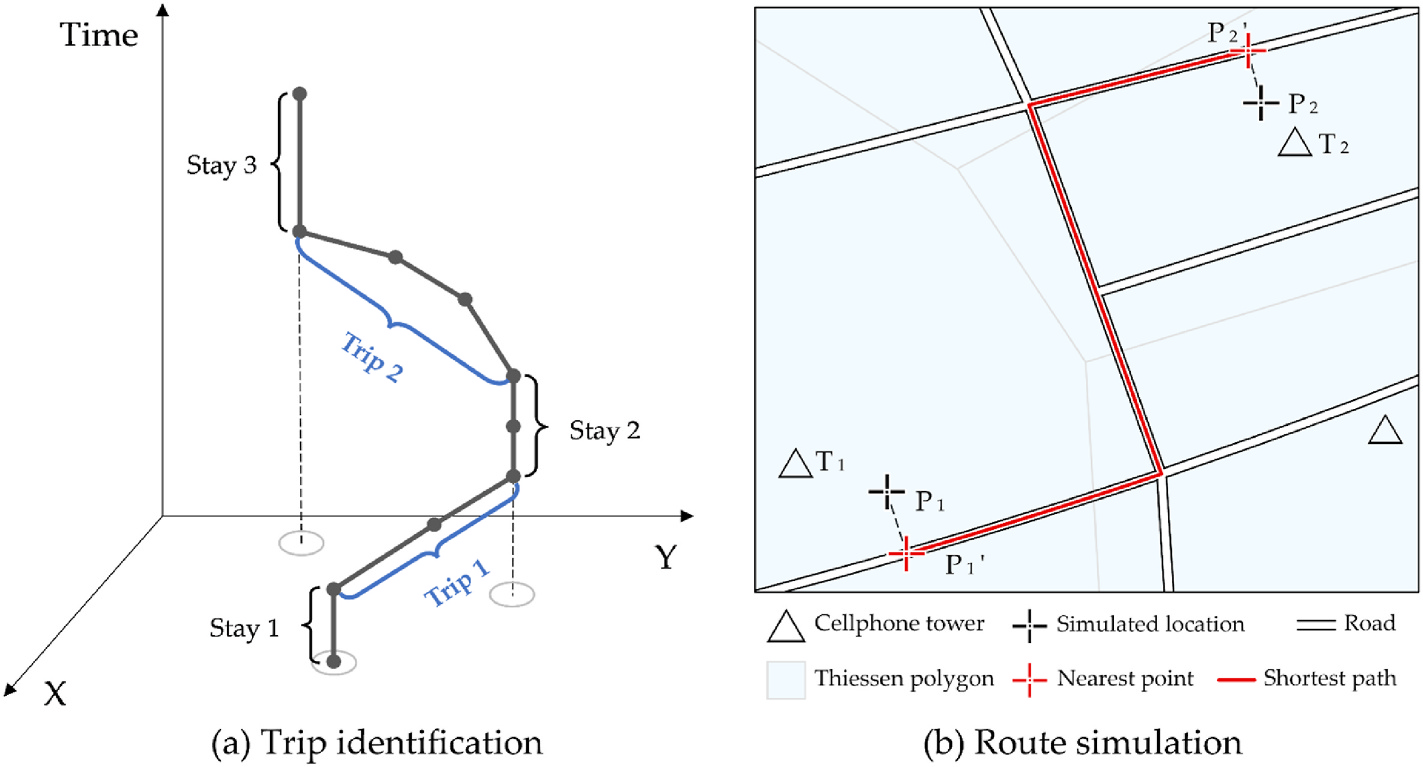
### 3.2. Trip identification and travel route simulation In this section, the trips of each cellphone user were identified and extracted from their trajectories. As shown in Fig. 6(a), we first detected the stay points of the user trajectories. If the distance between temporally consecutive records was less than a certain radius (e.g., 500 m), we considered them to be a stay point. When the user location shifts from one stay point to another, the trajectory between these two stay points is regarded as a trip (e.g., Trip 1 and Trip 2 in Fig. 6(a)). The origin and destination of this trip are represented by two Thiessen polygons (T₁ and T₂ in Fig. 6(b)), which indicate the service range of the corresponding cellphone tower. Because the cellphone location data do not contain travel routes between stay points, this study estimates the probable travel paths on the road network by using the shortest path algorithm (Dijkstra, 1959), which is a commonly used method to extract travel routes from cellphone data (Park, 2020). First, the starting and ending points for each trip (e.g., P₁ and P₂ in Fig. 6(b)) are simulated based on the Monte Carlo method (Strachan et al., 2007). The location points are randomly generated within the minimum bounding rectangle of the Thiessen polygon at each cellphone tower. The probability is set to 1 if the point is generated within the Thiessen polygon and otherwise is set to 0. After a series of random location point generation operations, the first point with a probability of 1 is set as the starting point or ending point. Second, the starting and ending points are associated with their closest roads, and the new starting and ending points are P′₁ and P′₂ (Fig. 6(b)), respectively. The user travel routes from P′₁ to P′₂ can be obtained by utilizing the shortest path algorithm. It is noted that trips are extracted only for individuals who move between stay points. Due to the insufficient spatial resolution of the cellphone location data, we cannot determine whether a user has moved if they are positioned at the same stay point for a continuous period. Therefore, trips within the range of stay points were not considered in this study. Finally, the number of users passing along each road is counted as the traffic flow on the road.

Figure 6. Example of trip identification and route simulation. — **Figure 6.** Example of trip identification and route simulation.

### 3.3. Estimating travel exposures of cellphone users For each user a, the cumulative travel exposure to on-road PM_2.5 for all n trips in a day can be calculated as follows:

Cum_TER_a = ∑_i=1ⁿ exposure_i (1)

where exposure_i represents the travel exposure of user a on the ith trip. It is described as follows:

exposure_i = ∑_j=1^m C_jT_j (2)

where m is the number of road segments that comprise the ith trip, C_j is the average PM_2.5 concentration on road segment j, and T_j is the travel time of user a on road segment j. Then, the average travel exposure for user a on their n trips during a certain period can be calculated as follows:

Ave_TER_a = Cum_TER_aT_a (3)

where T_a is the total travel time of user a for n trips. ## 4. Results We will analyse the results from the following three aspects. The first aspect concerns the assessment of each user’s travel exposures. The second aspect is to explore the patterns and characteristics of interpersonal variation in travel exposure. The third aspect is the analysis of the spatial heterogeneity of travel exposure at the road level across three periods. ### 4.1. 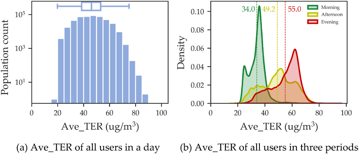Patterns and characteristics of users’ travel exposures Based on the methods introduced in section 3, we extracted the trips for each user and calculated their average travel exposure to on-road PM_2.5 (Ave_TER) during a day. Fig. 7(a) shows the distribution of the Ave_TER values for all users, which range from 5 μg/m³ to 90 μg/m³. For most users, the Ave_TER values are concentrated in the range of 20 μg/m³ to 75 μg/m³. Moreover, the average Ave_TER value for all users is 46.1 μg/m³, which is higher than the air quality guidance (24-h mean: 25 μg/m³ ) suggested by the WHO (World Health Organization, 2006). Fig. 7(b) shows the Ave_TER distributions of all users during three periods (e.g., morning, afternoon, and evening). The mean Ave_TER values in each period are marked with dashed vertical lines. In the morning, the Ave_TER value is less than 60 μg/m³, and the mean value is 34.0 μg/m³. In the afternoon, the variations in the Ave_TER values across users are larger, and the mean Ave_TER value is 49.2 μg/m³. In the evening, the Ave_TER value ranged from 20 μg/m³ to 80 μg/m³, with a mean value of 55.0 μg/m³. The Ave_TER value for all users in the morning is the lowest among the three periods, which is partly attributed to the lowest on-road PM_2.5 concentrations at that time. The Ave_TER ranges are similar in the afternoon and evening, whereas the mean Ave_TER of the latter is larger than that of the former. This is probably because the number of highly polluted roads is the highest in the evening, and people are more likely to be exposed to highly polluted road environments while travelling.

Figure 7. Distribution of the Ave_TER values of all users. — **Figure 7.** Distribution of the Ave_TER values of all users.

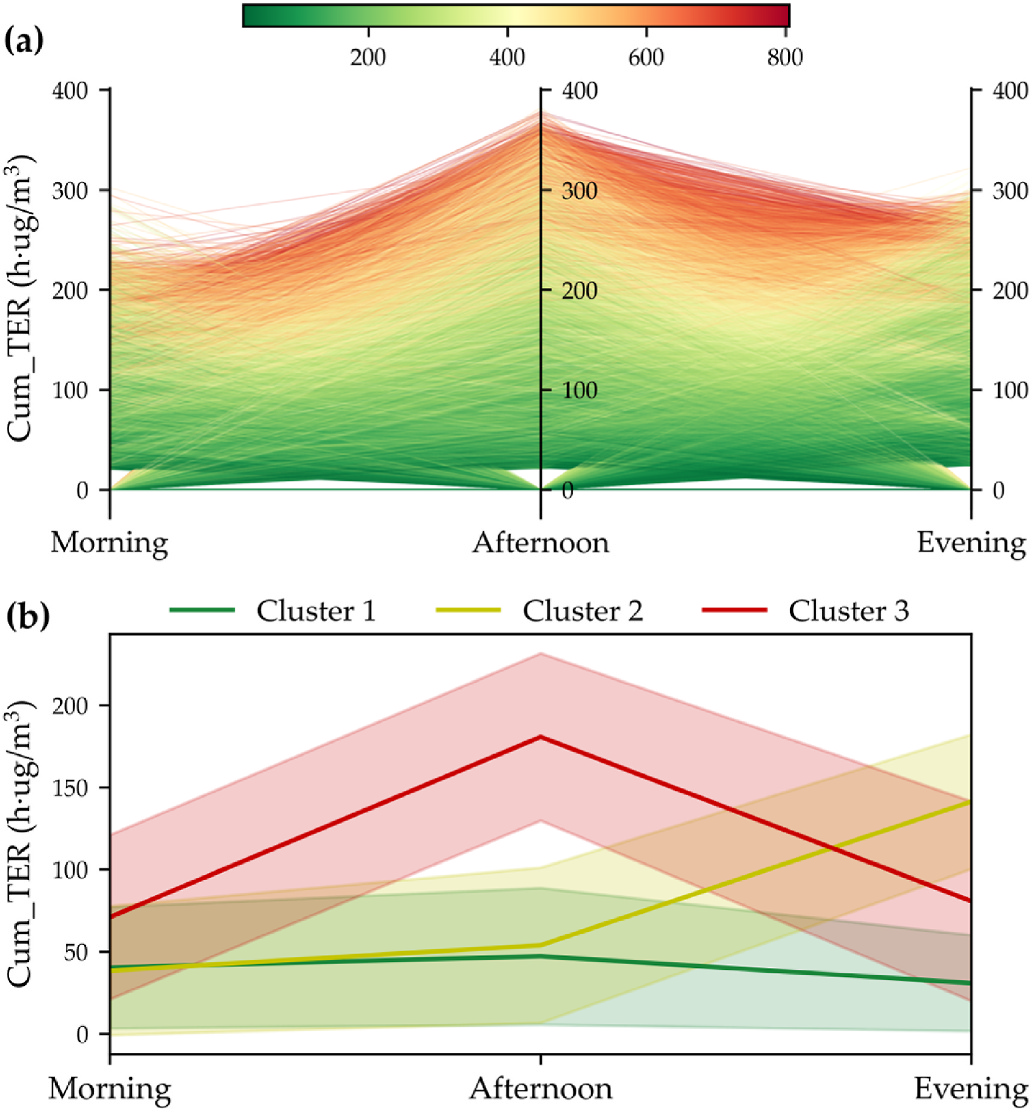
### 4.2. Interpersonal variations in travel exposure Fig. 8(a) shows the variations in the cumulative travel exposures (Cum_TER) for each user in the morning, afternoon, and evening periods. The maximum Cum_TER value occurs in the afternoon and approaches 350 h μg/m³, which is 5 times the average Cum_TER for all users during the same period. To explore the travel exposure patterns of all users, we further used a clustering method to explore the main temporal patterns of the individual travel exposures. We used a three-dimensional vector S = [Cum_TER_a^morning, Cum_TER_a^afternoon, Cum_TER_a^evening] to represent the travel exposure variations of user a in a day, where Cum_TER_a^morning, Cum_TER_a^afternoon, and Cum_TER_a^evening are the accumulated travel exposures of user a during n trips in the morning, afternoon, and evening, respectively. Then, the k-means algorithm was utilized to classify the S vectors of all users. The Calinski–Harabasz score was used to evaluate and determine the best k values. Higher Calinski–Harabasz score values indicate a better clustering result. We tested different values of k and found that the highest value of the Calinski–Harabasz score was obtained when k = 3. Therefore, the number of clusters is set to 3. After performing clustering, the percentages of users in Clusters 1, 2, and 3 are 54.0%, 25.5%, and 20.5%, respectively.

Figure 8. (a) The variations in Cum_TER values for each user in the morning, afternoon, and evening periods and (b) the temporal travel exposure patterns of three types of cellphone users. — **Figure 8.** (a) The variations in Cum_TER values for each user in the morning, afternoon, and evening periods and (b) the temporal travel exposure patterns of three types of cellphone users.

The curves representing the temporal travel exposure patterns of cellphone users who experience varying levels of exposure over the three defined periods are shown in Fig. 8(b). The thick solid line is the center of each cluster. The upper and lower borders of the coloured surface area are the mean values plus and minus the standard deviations, respectively. As shown in Fig. 8(b), the travel exposure patterns vary among users. For the users in Cluster 1, the Cum_TER in each period is the lowest compared with Clusters 2 and 3. Meanwhile, the standard deviations are the lowest, which indicates that the differences in the Cum_TER values among the users of Cluster 1 are less significant than those of Clusters 2 and 3. For the users in Clusters 2 and 3, the Cum_TER values in the three periods increase in the afternoon. The differences between Clusters 2 and 3 occur because the Cum_TER values of Cluster 2 rise further in the evening, whereas the Cum_TER values for Cluster 3 recover quickly after the afternoon period. This indicates that the high-risk time for Cluster 2 occurs in the evening, whereas the high-risk time for Cluster 3 occurs in the afternoon. Specifically, from the afternoon to evening, the Cum_TER values for Cluster 2 continue to increase from 50 h·μg/m³ to 120 h·μg/m³, but the Cum_TER values for Cluster 3 recover from 150 h·μg/m³ to 50 h·μg/m³. 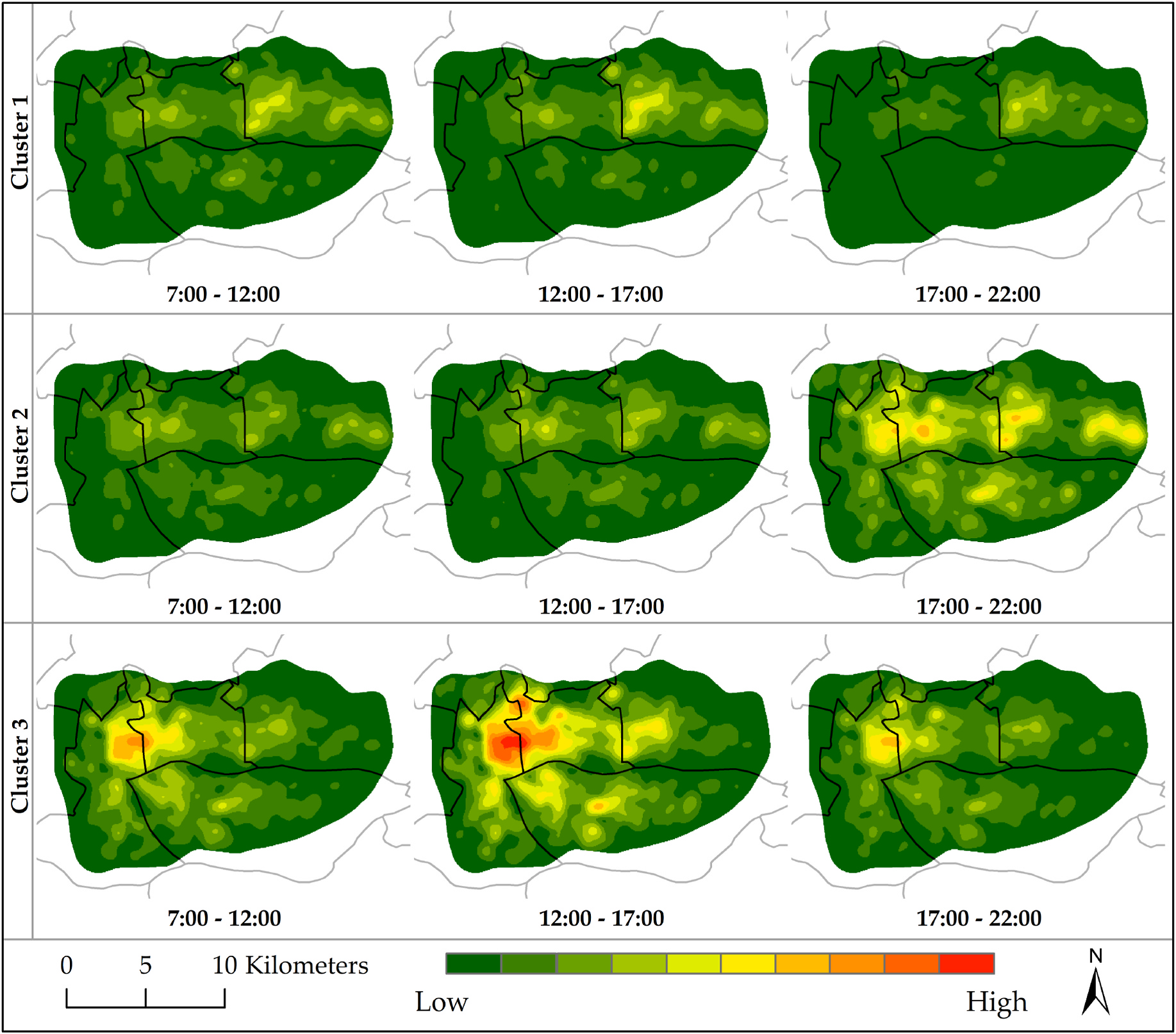We further examine the possible reasons why these three clusters of users have distinct travel exposure patterns from the perspective of their travel patterns. Fig. 9 shows the densities of the daily travel activities for each cluster. The users in Cluster 1 mainly travelled within the Tianhe district, where the on-road PM_2.5 concentrations were relatively low in all three periods. The users in Cluster 2 mainly travelled in the Yuexiu district, where the on-road PM_2.5 concentrations were very high in the evening. The users in Cluster 3 mainly travelled in the Yuexiu district and over a portion of the highly populated roads within Haizhu district. The travel activity intensity for Cluster 3 is particularly high in the middle of the day. These results suggest that the travel exposure patterns of residents are closely related to their daily travel habits. Through our study, the high-risk periods and high-risk roads for different populations are precisely pinpointed.

Figure 9. Daily travel patterns of three clusters of users. — **Figure 9.** Daily travel patterns of three clusters of users.

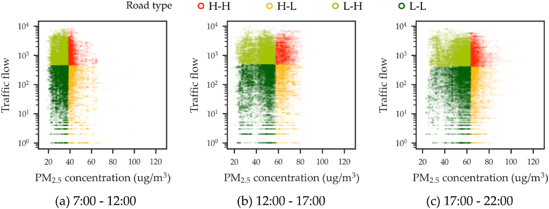
### 4.3. Spatial heterogeneity of travel exposure at the road level The spatial heterogeneity of the PM_2.5 concentrations on roads results in differences in their impacts on urban populations. Higher PM_2.5 concentrations and more travelers on a road indicate a higher risk. Fig. 10 displays the relationship between the PM_2.5 concentrations and traffic flows on the roads. For each period, the on-road PM_2.5 concentrations and traffic flows of all roads were ranked separately in descending order. Then, all roads are grouped by their rankings of the PM_2.5 concentrations and traffic flows. As shown in Fig. 10, the red symbols represent the roads with the highest 25% PM_2.5 concentrations and traffic flows, which are called H–H type roads. The orange symbols represent the roads with the highest 25% of PM_2.5 concentrations and lowest 75% of traffic flows, which are H–L type roads. The mustard symbols represent the roads with the lowest 75% of PM_2.5 concentrations and highest 25% of traffic flow, which are called L–H type roads. The roads depicted in green have the lowest 75% PM_2.5 concentrations and traffic flows and are called L–L type roads.

Figure 10. Types of roads grouped by PM2.5 concentrations and traffic flows. — **Figure 10.** Types of roads grouped by PM_2.5 concentrations and traffic flows.

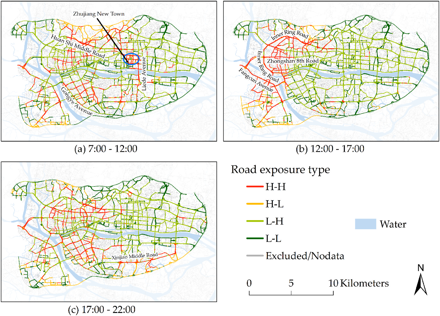
The spatial distributions of the four road types are shown in Fig. 11. The locations of the four types of roads are not stable over time, which is related to the distributions of the on-road PM_2.5 concentrations and travel activity intensities at different times of the day. Since the H–H road type affects a large number of travelers, we thus use this as an example to analyse its characteristics. In the morning, the H–H type roads are mainly concentrated in three areas, such as Huan Shi Middle Road, Liede Avenue and the roads around Zhujiang New Town, and Industrial Avenue. In the afternoon, the H–H type roads are mainly located in the left part of the study area, such as Fangcun Avenue, Inner Ring Road, and Zhongshan 8th Road. In the evening, the H–H type roads are more dispersed in space. In addition to the roads highlighted in the morning, Xinjiao Middle Road also becomes an H–H type road in the evening. The H–L type roads have lower traffic volumes despite having very high PM_2.5 concentrations and thus affect fewer travelers. Therefore, the government should focus more on H–H type roads and decrease the risk of PM_2.5 exposure of people on H–H type roads by using travel route guidance and environmental improvements. The vulnerable populations can modify their travel plans or try to avoid going outdoors during the peak concentration hours and travelling on highly polluted roads.

Figure 11. Spatial distributions of the four road types. — **Figure 11.** Spatial distributions of the four road types.

## 5. Discussion In our study, the travel routes of cellphone users were simulated by using the shortest path algorithm under the assumption that people choose the shortest paths to travel in most cases. Since the actual travel routes are not available in the cellphone positioning data, there is a lack of “ground truth” data to validate our results. To evaluate whether the users’ travel exposures can be seriously biased under the shortest path assumption, we designed more experiments to quantify the differences in users’ travel exposure to on-road PM_2.5 by comparing the shortest-path (SP) strategy with two other route choice strategies. They are defined as follows: - **Random-path (RP) strategy:** users randomly choose one path from the k shortest paths. - **Longest-path (LP) strategy:** users choose the longest path from the k shortest paths. The SP strategy is viewed as the base strategy. For the RP and LP strategies, we used the k shortest path algorithm (Eppstein, 1998) to obtain the top k shortest paths for each origin-destination pair. If k is sufficiently large, the k shortest paths can theoretically include all the travel route options of users. To lower the computational time, we have to choose a reasonable k value first. 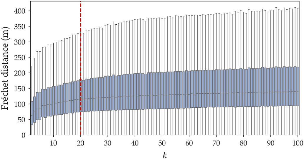The Fréchet distance (Alt and Godau, 1995; Devogele et al., 2017), a measure of similarity between curves that takes into account the location and ordering of the points along the curves, was used to measure the similarity of the kth shortest path and the shortest path. As shown in Fig. 12, the Fréchet distance ascends slowly as k increases from 2 to 100. When k is greater than 20, the Fréchet distance varies slightly, which means that the similarity of the kth shortest path and the shortest path will no longer change dramatically. The optimal k value is set to 20 by considering the computational time and the stability of the results.

Figure 12. Distributions of Fréchet distance of all users with different values of k. — **Figure 12.** Distributions of Fréchet distance of all users with different values of `k`.

Then, we randomly selected 5000 cellphone users and evaluated the travel exposure difference between the RP strategy and SP strategy as k increases from 2 to 20. The percentage difference in the cumulative travel exposure (Diff_Exposure) of user a between RP and SP strategy was calculated as follows:

Diff_Exposure_a(i) = Cum_TER_a(i) − Cum_TER_a(1)Cum_TER_a(1) × 100%, 1 ≤ i ≤ k (4)

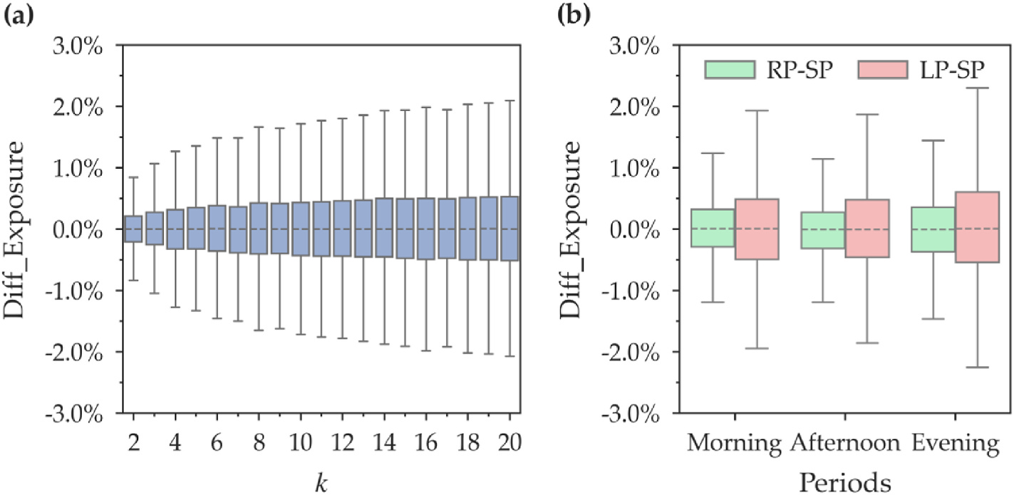
where Cum_TER_a(i) is the cumulative travel exposure of user a when he/she chooses the ith shortest path from the k shortest paths. Fig. 13(a) shows the distribution of Diff_Exposure of all users at different k values. It is found that the median Diff_Exposure always remains at 0 when k increases from 2 to 20. By investigating the relationship of Diff_Exposure with k, we find that a larger k value tends to generate greater travel exposure differences. The 1.5 interquartile range (1.5IQR) reaches the maximum when k is 20, and the maximum and minimum Diff_Exposure between the RP strategy and SP strategy are 2.0 and −2.0%, respectively. This means that the over- or under-estimation of users’ travel exposures is within a small range, even though users’ travel routes do not necessarily follow the shortest paths. In three periods, the distributions of Diff_Exposure between LP and SP and between RP and SP strategy, are further assessed to examine the upper and lower bounds of Diff_Exposure across different times of the day. Fig. 13(b) shows that the median of Diff_Exposure between LP and SP strategy is approximately 0 over three periods. The 1.5IQR reaches the maximum in the evening, and the lower and upper bounds of Diff_Exposure are −2.5% and 2.5%, respectively. Similarly, the range within 1.5IQR of Diff_Exposure between RP and SP strategy also reaches the maximum in the evening, and the lower and upper bounds are −1.5% and 1.5%, respectively. By comparing these two distributions of Diff_Exposure, we find that the maximum difference in users’ travel exposures occurs in the evening for both the SP and LP strategies, whereas the LP strategy generates greater exposure estimation differences.

Figure 13. Boxplots of Diff_Exposure distribution (a) for different k values, (b) across different periods (whiskers indicate 1.5 interquartile range (1.5IQR)). — **Figure 13.** Boxplots of Diff_Exposure distribution (a) for different `k` values, (b) across different periods (whiskers indicate 1.5 interquartile range (1.5IQR)).

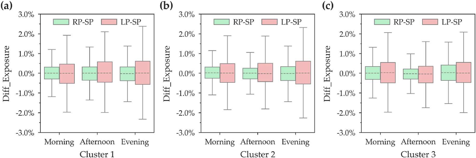
In section 4, all users were classified into three clusters with distinct travel exposure patterns. Therefore, we compared the distribution of Diff_Exposure among the three clusters of users to quantify the travel exposure differences of each type of users if they choose travel paths using the RP or LP strategy (Fig. 14). For the three clusters of users, the distribution of Diff_Exposure among them had a similar trend: the LP strategy generates greater exposure estimation differences than the RP strategy, and the IQR and 1.5IQR of Diff_Exposure between LP and SP strategy are larger than those between RP and SP strategy in all three periods. For users in cluster 1, the 1.5IQR of Diff_Exposure between LP and SP rises from morning to evening, and the lower and upper bounds of Diff_Exposure are −2.5% and 2.5%, respectively. For the users of cluster 2, the 1.5IQR of Diff_Exposure between LP and SP in the afternoon is less than that in the other two periods. The largest 1.5IQR appears in the evening, with lower and upper bounds of −2.5% and 2.5%, respectively. For users in cluster 3, the largest 1.5IQR of Diff_Exposure between LP and SP is in the morning, with lower and upper bounds of −2.0% and 2.0%, respectively.

Figure 14. Distributions of Diff_Exposure of three clusters of users. — **Figure 14.** Distributions of Diff_Exposure of three clusters of users.

Overall, the travel exposure differences between LP and SP and between RP and SP strategy vary across users and periods. The maximum travel exposure difference is no more than 2.5%, even if all users choose the LP strategy for travelling. Therefore, we can conclude that the biases introduced by the shortest path assumption are kept to a reasonable level. Even though users do not exactly follow the shortest paths, the estimation of travel exposure does not vary that much. ## 6. Conclusions PM_2.5 pollution has imposed substantial health risks on urban residents. Previous studies mainly focused on assessing peoples’ exposure at static locations, such as homes or workplaces. However, there has been a scarcity of research that quantifies the dynamic PM_2.5 exposures of people when they travel in cities. In this study, we used cellphone positioning data and PM_2.5 concentration data that were collected by using smart sensors along roads in Guangzhou, China, to assess the travel exposures of individuals to on-road PM_2.5. First, we extracted the trips of the cellphone users from their trajectories and estimated their travel routes on the road network by using the shortest path algorithm. Then, we estimated the travel exposure of each user by associating their movement patterns with PM_2.5 concentrations on roads. In our study, the PM_2.5 concentration data on roads were collected by using mobile sensors. Compared with air pollution data obtained using fixed monitoring stations and remote sensing monitoring methods, the data obtained from roads can more accurately reflect the air quality in the daily travel environments of urban residents. Moreover, unlike the studies that are based on limited travel survey samples, this study was able to assess the overall travel exposure of a large urban population. The results show that travel exposure cannot be ignored when providing a more comprehensive assessment of the air pollution exposure of urban residents. For most cellphone users in Guangzhou, China, the average travel exposure per hour falls within the range of 20 μg/m³ to 75 μg/m³. The most severe travel exposures occur in the evening, with a mean value of 55.0 μg/m³. There are three types of users who experience varying levels of exposure over the three defined periods. The users in Cluster 1 (54.0%) experience low travel exposures throughout the day. The high-risk time for users in Cluster 2 (25.5%) occurred in the evening, whereas the high-risk time for users in Cluster 3 occurred in the afternoon (20.5%). Furthermore, it is found that the impacts of on-road PM_2.5 on urban populations are uneven across roads, and more attention should be given to roads with high PM_2.5 concentrations and traffic flows in each period, such as Huan Shi Middle Road in the morning, Inner Ring Road in the afternoon, and Xinjiao Middle Road in the evening. The findings in this study can contribute to a more in-depth understanding of the relationship between air pollution and travel activities of the urban population. Additionally, it can provide targeted policies and valuable suggestions for the government and individuals to reduce the health risk caused by on-road PM_2.5 pollution. There are a few limitations of this study. First, despite the potential of cellphone data to assess air pollution exposures in large populations, the spatial and temporal resolutions of the cellphone data used in this study are relatively low compared with those of GPS data. Thus, some short trips within the service range of each cellphone tower might be filtered out. Second, since actual travel routes are not available in the cellphone data, they were estimated by using shortest path algorithms. However, in reality, users’ travel routes do not necessarily follow the shortest paths (Park, 2020), which might overestimate or underestimate users’ travel exposure. According to our evaluation, the median values of travel exposure differences are almost 0% in all three periods. The maximum travel exposure differences are no more than 2.5%, which means even if each user chooses the longest path for travelling, the estimation of travel exposure does not vary that much. Third, the actual utilizations of different travel modes (e.g., car, bus, bicycle, or walking) were not considered because the user travel modes were not recorded in the cellphone data. These modes cannot be accurately inferred due to the limitations of cellphone data (Huang et al., 2019a,b). Therefore, the exposure assessment results can be affected to a certain extent. Fourth, because of labor costs, the use of cyclists to collect on-road PM_2.5 data has difficulties in capturing the day-to-day variability and seasonal variability of urban air pollution. However, it is still an attempt to obtain large-scale and high-resolution PM_2.5 data. In the future, we will try to collect on-road PM_2.5 concentration data covering more days to make it more representative. Nevertheless, this research contributes to personal travel exposure assessment from a dynamic perspective by combining field-collected on-road PM_2.5 concentration data and individuals’ travel routes extracted from large-scale cellphone data. ## Acknowledgements This work was supported by National Natural Science Foundation of China [grant number 41971345, 71961137003, 42011530172]; Guangdong Basic and Applied Basic Research Foundation [grant number 2020A1515010695]. ## References - Alt, H., Godau, M., 1995. Computing the Fréchet distance between two polygonal curves. Int. J. Comput. Geom. Appl. 5 (1), 75–91. - Andersson, J., Oudin, A., Nordin, S., Forsberg, B., Nordin, M., 2021. PM2.5 exposure and olfactory functions. Int. J. Environ. Health Res. [https://doi.org/10.1080/09603123.2021.1973969](https://doi.org/10.1080/09603123.2021.1973969). - Birenboim, A., Helbich, M., Kwan, M.-P., 2021. Advances in portable sensing for urban environments: understanding cities from a mobility perspective. Comput. Environ. Urban Syst. 88. - Bowatte, G., Lodge, C., Lowe, A.J., Erbas, B., Perret, J., Abramson, M.J., Matheson, M., Dharmage, S.C., 2015. The influence of childhood traffic-related air pollution exposure on asthma, allergy and sensitization: a systematic review and a meta-analysis of birth cohort studies. Allergy Eur. J. Allergy Clin. Immunol. 70, 245–256. - Chen, H., Goldberg, M.S., Viileneuve, P.J., 2008. A systematic review of the relation between long-term exposure to ambient air pollution and chronic diseases. Rev. Environ. Health 23, 243–297. - China Vehicle Environmental Management Annual Report, 2018. Ministry of Ecology and Environment of the People’s Republic of China, Beijing. - Cohen, A.J., Brauer, M., Burnett, R., Anderson, H.R., Frostad, J., Estep, K., Balakrishnan, K., Brunekreef, B., Dandona, L., Dandona, R., Feigin, V., Freedman, G., Hubbell, B., Jobling, A., Kan, H., Knibbs, L., Liu, Y., Martin, R., Morawska, L., Pope III, C.A., Shin, H., Straif, K., Shaddick, G., Thomas, M., van Dingenen, R., van Donkelaar, A., Vos, T., Murray, C.J.L., Forouzanfar, M.H., 2017. Estimates and 25-year trends of the global burden of disease attributable to ambient air pollution: an analysis of data from the Global Burden of Diseases Study 2015. Lancet 389, 1907–1918. - Devogele, T., Etienne, L., Esnault, M., Lardy, F., 2017. Optimized discrete Fréchet distance between trajectories. In: Proceedings of the 6th ACM SIGSPATIAL Workshop on Analytics for Big Geospatial Data, BigSpatial’17. - Dewulf, B., Neutens, T., Lefebvre, W., Seynaeve, G., Vanpoucke, C., Beckx, C., Van de Weghe, N., 2016. Dynamic assessment of exposure to air pollution using mobile phone data. Int. J. Health Geogr. 15, 1–14. [https://doi.org/10.1186/s12942-016-0042-z](https://doi.org/10.1186/s12942-016-0042-z). - Dijkstra, E.W., 1959. A note on two problems in connexion with graphs. Numer. Math. 1, 269–271. - Dominici, F., Peng, R.D., Bell, M.L., Pham, L., McDermott, A., Zeger, S.L., Samet, J.M., 2006. Fine particulate air pollution and hospital admission for cardiovascular and respiratory diseases. J. Am. Med. Assoc. 295, 1127–1134. - Eppstein, D., 1998. Finding the k shortest paths. SIAM J. Comput. 28 (2), 652–673. - Guangzhou Statistical Yearbook, 2018. Guangzhou Municipal Bureau of Statistics and Guangzhou Survery Office of National Bureau of Statisitcs. - Gulliver, J., Briggs, D.J., 2005. Time-space modeling of journey-time exposure to traffic-related air pollution using GIS. Environ. Res. 97, 10–25. - Guo, H., Li, W., Yao, F., Wu, J., Zhou, X., Yue, Y., Yeh, A.G.O., 2020. Who are more exposed to PM2.5 pollution: a mobile phone data approach. Environ. Int. 143. - He, Q., Zhang, M., Song, Y., Huang, B., 2021. Spatiotemporal assessment of PM2.5 concentrations and exposure in China from 2013 to 2017 using satellite-derived data. J. Clean. Prod. 286. - Hoteit, S., Secci, S., Sobolevsky, S., Ratti, C., Pujolle, G., 2014. Estimating human trajectories and hotspots through mobile phone data. Comput. Network. 64, 296–307. - Huang, G., Zhou, W., Qian, Y., Fisher, B., 2019a. Breathing the same air? Socioeconomic disparities in PM2.5 exposure and the potential benefits from air filtration. Sci. Total Environ. 657, 619–626. - Huang, H., Cheng, Y., Weibel, R., 2019b. Transport mode detection based on mobile phone network data: a systematic review. Transport. Res. C Emerg. Technol. 101, 297–312. - Kwan, M.-P., Liu, D., Vogliano, J., 2015. Assessing dynamic exposure to air pollution. In: Space-Time Integration in Geography and GIScience. Springer, Dordrecht, pp. 283–300. - Li, M., Gao, S., Lu, F., Tong, H., Zhang, H., 2019. Dynamic estimation of individual exposure levels to air pollution using trajectories reconstructed from mobile phone data. Int. J. Environ. Res. Publ. Health 16, 4522. - Li, Q., Zou, D., Xu, Y., 2021. Combining individual travel behaviour and collective preferences for next location prediction. Transportmetrica A: Transport. Sci. [https://doi.org/10.1080/23249935.2021.1968066](https://doi.org/10.1080/23249935.2021.1968066). - Liu, Z., Xie, M., Tian, K., Gao, P., 2017. GIS-based analysis of population exposure to PM2.5 air pollution—a case study of Beijing. J. Environ. Sci. 59, 48–53. - Ma, J., Tao, Y., Kwan, M.-P., Chai, Y., 2020. Assessing mobility-based real-time air pollution exposure in space and time using smart sensors and GPS trajectories in Beijing. Ann. Assoc. Am. Geogr. 110, 434–448. - Ministry of Environmental Protection, 2013. Technical Regulation for Selection of Ambient Air Quality Monitoring Stations (On Trial), 2013-09-22. - Nyhan, M., Grauwin, S., Britter, R., Misstear, B., McNabola, A., Laden, F., Barrett, S.R.H., Ratti, C., 2016. Exposure track” - the impact of mobile-device-based mobility patterns on quantifying population exposure to air pollution. Environ. Sci. Technol. 50, 9671–9681. [https://doi.org/10.1021/acs.est.6b02385](https://doi.org/10.1021/acs.est.6b02385). - Nyhan, M.M., Kloog, I., Britter, R., Ratti, C., Koutrakis, P., 2019. Quantifying population exposure to air pollution using individual mobility patterns inferred from mobile phone data. J. Expo. Sci. Environ. Epidemiol. 29, 238–247. - Ouyang, W., Gao, B., Cheng, H., Hao, Z., Wu, N., 2018. Exposure inequality assessment for PM2.5 and the potential association with environmental health in Beijing. Sci. Total Environ. 635, 769–778. - Park, Y.M., 2020. Assessing personal exposure to traffic-related air pollution using individual travel-activity diary data and an on-road source air dispersion model. Health Place 63. - Piedrahita, R., Xiang, Y., Masson, N., Ortega, J., Collier, A., Jiang, Y., Li, K., Dick, R.P., Lv, Q., Hannigan, M., Shang, L., 2014. The next generation of low-cost personal air quality sensors for quantitative exposure monitoring. Atmos. Meas. Tech. 7, 3325–3336. - Song, J., Zhou, S., Xu, J., Su, L., 2021. From PM2.5 exposure to PM2.5 risks of inhaled dose in daily activities: empirical evidence during workdays from guangzhou, China. Atmos. Environ. 249. - Song, Y., Huang, B., He, Q., Chen, B., Wei, J., Mahmood, R., 2019. Dynamic assessment of PM2.5 exposure and health risk using remote sensing and geo-spatial big data. Environ. Pollut. 253, 288–296. - Strachan, S., Williamson, J., Murray-Smith, R., 2007. Show me the way to Monte Carlo: density-based trajectory navigation. In: Conf Hum Fact Comput Syst Proc. Presented at the 25th SIGCHI Conference on Human Factors in Computing Systems 2007, CHI 2007, pp. 1245–1248. San Jose, CA. - U.S. Environmental Protection Agency, 2012. Revised Air Quality Standards for Particle Pollution and Updates to the Air Quality Index (AQI). - Wong, D.W., Yuan, L., Perlin, S.A., 2004. Comparison of spatial interpolation methods for the estimation of air quality data. J. Expo. Anal. Environ. Epidemiol. 14, 404–415. - World Health Organization, 2006. Air Quality Guidelines: Global Update 2005: Particulate Matter, Ozone, Nitrogen Dioxide, and Sulfur Dioxide. World Health Organization. - Wu, J., Wilhelm, M., Chung, J., Ritz, B., 2011. Comparing exposure assessment methods for traffic-related air pollution in an adverse pregnancy outcome study. Environ. Res. 111, 685–692. - Xu, Y., Jiang, S., Li, R., Zhang, J., Zhao, J., Abbar, S., González, M.C., 2019. Unravelling environmental justice in ambient PM2.5 exposure in Beijing: a big data approach. Comput. Environ. Urban Syst. 75, 12–21. - Xu, Y., Li, X., Shaw, S.-L., Lu, F., Yin, L., Chen, B.Y., 2020. Effects of data preprocessing methods on addressing location uncertainty in mobile signaling data. Ann. Assoc. Am. Geogr. 111, 515–539. - Yin, M., Sheehan, M., Feygin, S., Paiement, J.-F., Pozdnoukhov, A., 2018. A generative model of urban activities from cellular data. IEEE Trans. Intell. Transport. Syst. 19, 1682–1696. - Yoo, E.H., Rudra, C., Glasgow, M., Mu, L., 2015. Geospatial estimation of individual exposure to air pollutants: moving from static monitoring to activity-based dynamic exposure assessment. Ann. Assoc. Am. Geogr. 105, 915–926. [https://doi.org/10.1080/00045608.2015.1054253](https://doi.org/10.1080/00045608.2015.1054253). - Yu, H., Russell, A., Mulholland, J., Huang, Z., 2018. Using cell phone location to assess misclassification errors in air pollution exposure estimation. Environ. Pollut. 233, 261–266. - Zhou, S., Lin, R., 2019. Spatial-temporal heterogeneity of air pollution: the relationship between built environment and on-road PM2.5 at micro scale. Transport. Res. Transport Environ. 76, 305–322.